Diagnostics
12/16/2017
A Data Set & Model
The Data
Independent observations with two possible outcomes on a trial.
Use ggplot to generate a data graph showing successes, failures, and total observations. 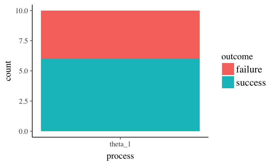
The Model
A graphical representation of the model shows:
- a continuous, unobserved “process” parameter \(\theta\)
- a discrete, observable number of successes k
- a discrete, observable number of observations n
The vector’s arrow shows dependency. Successes are dependent on both the underlying process \(\theta\) and the number of observations.
The assumption for \(\theta\) is that all possible rates are equally likely. The Beta distribution is set with 1 “success” and 1 “failure”.
The assumption of k is that the outcomes are from a Binomial distribution with \(\theta\) determining the rate for n observations.
Basic Stan Output
Extract information from a S4 object of class stanfit.
Use get_stancode to extract the model from the stan output.
## // Infering a Rate "theta" of a binary process
## // Section 3.1
## // Figure 3.2
## data {
##   int<lower=1> n; // at least one observation
##   int<lower=0> k; // success count can not be negative
## }
##
## parameters {
##   real<lower=0, upper=1> theta; // rate bounded by 0 and 1
## }
##
## model {
##   //Prior Distribution for Rate Theta
##   theta ~ beta(1, 1);
##
##   // Observed Counts
##   // k has a binomial distribution of n observations with theta variation
##   k ~ binomial(n, theta);
## }
Print on a stanfit object shows summary of the model fit:
- first parameter is “theta”
- second parameter is “lp__" - the log posterior density
- se_mean is the Monte Carlo standard error
- n_eff is the effective sample size
- Rhat is the R-hat statistic
Convergence of log posterior density is critical to declaring convergence (see stan-reference-2.16.0.pdf pg 368-369).
## Inference for Stan model: binomial_one_rate.
## 4 chains, each with iter=2000; warmup=1000; thin=1;
## post-warmup draws per chain=1000, total post-warmup draws=4000.
##
##        mean se_mean   sd   2.5%   25%   50%   75% 97.5% n_eff Rhat
## theta  0.58    0.00 0.14   0.30  0.48  0.59  0.68  0.83  1281    1
## lp__  -8.69    0.02 0.78 -10.86 -8.88 -8.40 -8.21 -8.15  1738    1
##
## Samples were drawn using NUTS(diag_e) at Sat Dec 16 12:36:37 2017.
## For each parameter, n_eff is a crude measure of effective sample size,
## and Rhat is the potential scale reduction factor on split chains (at
## convergence, Rhat=1).
Diagnostics
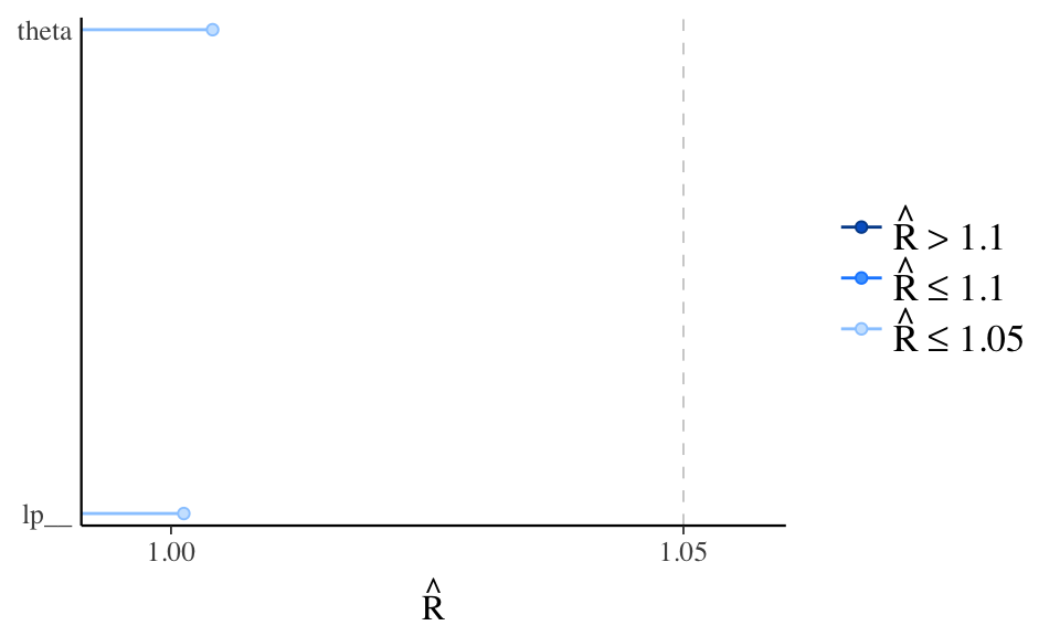
Rhat - potential scale reduction statistic
If chains are at equilibrium, rhat will be 1. If the chains have not converged rhat will be greater than one.
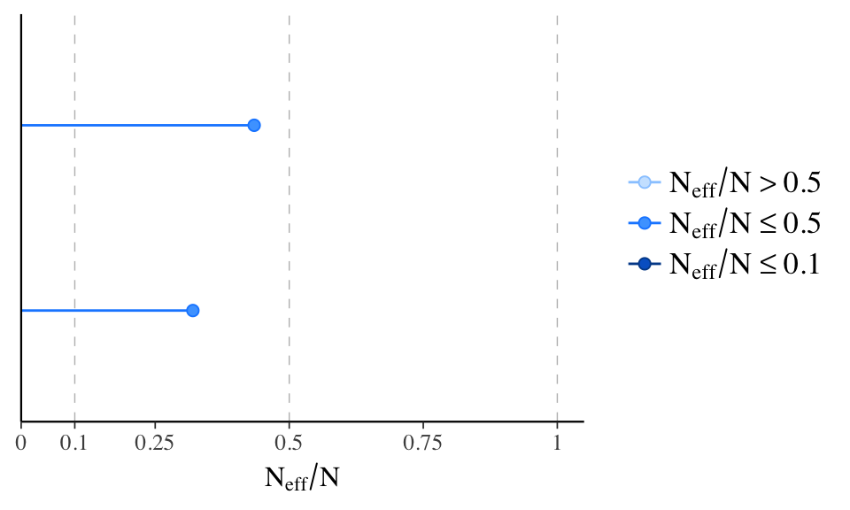
neff_ratio - Look at effective sample size
Draws in a Markov chain are not independent if there is autocorrelation. If there is autocorrelation, the effective sample size will be smaller than the total sample size, N.
The larger the ratio of neff to N the better.
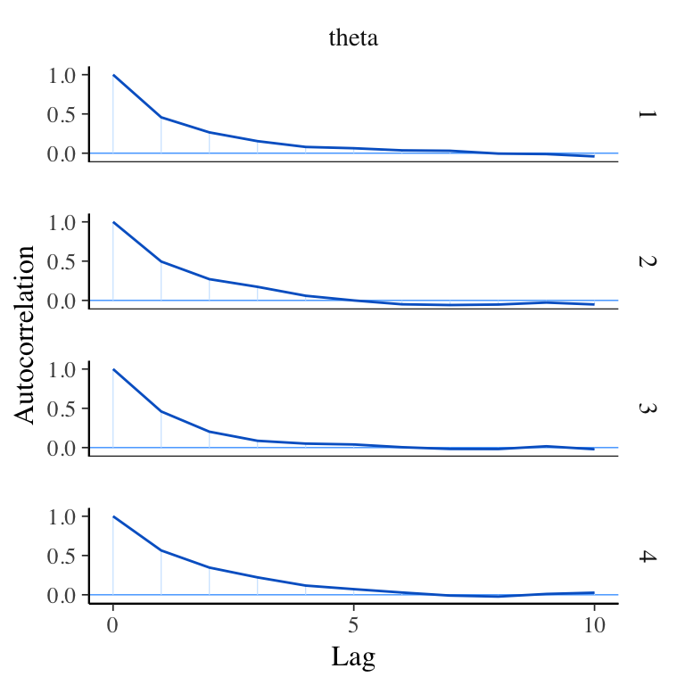
mcmc_acf - Autocorrelation Function
View autocorrelation for each Markov chain separately up to a specified number of lags.
Lag - the distance between successive samples.
The autocorrelation function (ACF) relates correlation and lag. The values of the ACF should quickly decrease with increasing lag. ACFs that do not decrease quickly with lag often indicate that the sampler is not exploring the posterior distribution efficiently and result in increased R^ values and decreased Neff values. (See Bayesian inference with Stan: A tutorial on adding custom distributions).
Evaluate NUTS sampler
Extract the log posterior (i.e., log_posterior(samples) ) and iterations with divergence (i.e., nuts_params(samples) ) from the stan output.
Trace plot of MCMC draws and divergence, if any, for NUTS.
## No divergences to plot.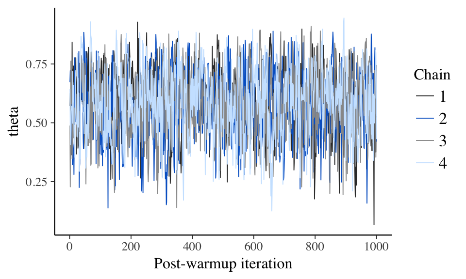
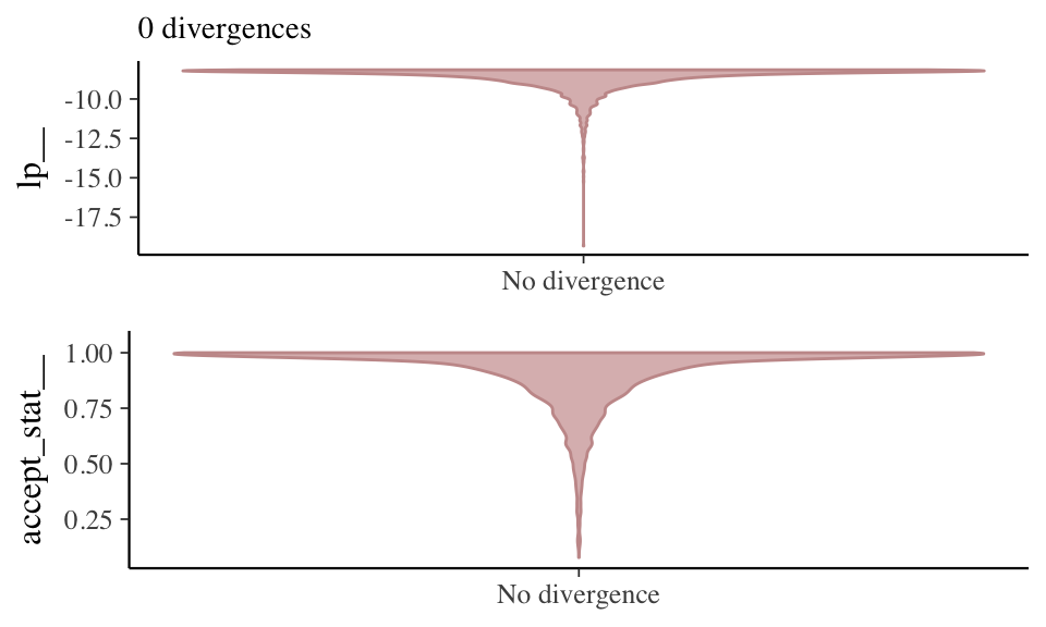
A different look at divergence.
Divergences often indicate that some part of the posterior isn’t being explored. Divergence shows as distortions in the smooth funnel.
Other Diagnostics & Graphs
A more detailed summary using the summary() function.
## $summary
##             mean     se_mean        sd        2.5%        25%        50%
## theta  0.5799059 0.003901466 0.1396456   0.2990563  0.4825571  0.5862972
## lp__  -8.6939063 0.018687798 0.7791654 -10.8626288 -8.8791850 -8.4005691
##              75%      97.5%    n_eff     Rhat
## theta  0.6813911  0.8339296 1281.147 1.004059
## lp__  -8.2063674 -8.1509108 1738.373 1.001246
##
## $c_summary
## , , chains = chain:1
##
##          stats
## parameter       mean        sd        2.5%        25%       50%        75%
##     theta  0.5825189 0.1330357   0.3225311  0.4926727  0.589468  0.6732102
##     lp__  -8.6404990 0.7498039 -10.4428005 -8.8192743 -8.352550 -8.1971973
##          stats
## parameter     97.5%
##     theta  0.820949
##     lp__  -8.150525
##
## , , chains = chain:2
##
##          stats
## parameter       mean        sd       2.5%        25%        50%        75%
##     theta  0.5722978 0.1417743   0.279753  0.4734228  0.5796229  0.6756787
##     lp__  -8.7065085 0.7814133 -10.907407 -8.8882874 -8.4139222 -8.2092875
##          stats
## parameter      97.5%
##     theta  0.8325598
##     lp__  -8.1511338
##
## , , chains = chain:3
##
##          stats
## parameter       mean       sd        2.5%       25%       50%        75%
##     theta  0.5774489 0.138483   0.2964121  0.477725  0.583742  0.6772734
##     lp__  -8.6824826 0.745806 -10.8626288 -8.838242 -8.400059 -8.2101127
##          stats
## parameter     97.5%
##     theta  0.835351
##     lp__  -8.151059
##
## , , chains = chain:4
##
##          stats
## parameter       mean        sd        2.5%        25%        50%
##     theta  0.5873577 0.1447749   0.3059745  0.4852965  0.5919105
##     lp__  -8.7461351 0.8338485 -10.9892909 -8.9576793 -8.4321885
##          stats
## parameter        75%      97.5%
##     theta  0.6898992  0.8406215
##     lp__  -8.2110721 -8.1510385
Other Functions to run on stanfit object
- stan_trace(samples)
- stan_hist(samples)
- stan_dens(samples)
- stan_scat(samples)
- stan_diag(samples)
- stan_rhat(samples)
- stan_ess(samples)
- stan_mcse(samples)
- stan_ac(samples)
Copyright © 2017 OBrien Consulting - All rights reserved.